TDCSLIST
Describes the electrode positions, shapes, currents as well as conductivity information for a single tDCS simulation.
Initialization
Python
from simnibs import sim_struct
s = sim_struct.SESSION()
tdcs_list = s.add_tdcslist()
MATLAB
s = sim_struct('SESSION');
tdcs_list = sim_struct('TDCSLIST');
s.poslist{1} = tdcs_list;
Attributes
currents list/array of floats (Python/MATLAB)
Description: Current values (in Ampere), must sum to zero
Example: Python/MATLAB
tdcs_list.currents = [1e-3, -1e-3]
Note: Currents are given per channel, not per electrode. Please see the ELECTRODE structure documentation for more information
electrode: list/array of ELECTRODE structures (Python/MATLAB)
Description: List containing the electrodes to be used for the simulations.
Note: Please see the ELECTRODE structure documentation for more information
cond: list/array of COND structures (Python/MATLAB), optional
Description: List containing the tissue names and conductivities
Default: Standard conductivity values
Example:
Python
# Change White Matter conductivity to 0.1 S/m
# Notice, we need to reduce the tissue number by 1
# in order to make up for the fact that python
# indexing starts at zero
tdcs_list.cond[0].value = 0.1
MATLAB
% Change White Matter conductivity to 0.1 S/m
tdcs_list.cond(1).value = 0.1;
Note: Please see the COND structure documentation for more information. All electrodes will get their conductivities from the tissues 100 and 500.
anisotropy_type: ‘scalar’, ‘vn’, ‘dir’ or ‘mc’, optional
Description: Type of conductivity values to use in gray and white matter.
‘scalar’: Isotropic, piecewise-constant conductivity values (default)
‘vn’: Volume normalized anisotropic conductivities. In the volume normalization process, tensors are normalized to have the same trace and re-scaled according to their respective tissue conductivitiy (recommended for simulations with anisotropic conductivities, see Opitz et al., 2011)
‘dir’: Direct anisotropic conductivity. Does not normalize individual tensors, but re-scales them accordingly to the mean gray and white matter conductivities (see Opitz et al., 2011).
‘mc’: Isotropic, varying conductivities. Assigns to each voxel a conductivity value related to the volume of the tensors obtained from the direct approach (see Opitz et al., 2011).
Default: ‘scalar’
Note: All options other than ‘scalar’ require conductivity tensors acquired from diffusion weighted images and processed with dwi2cond.
Reference: Tuch et al., 2001, Opitz et al., 2011
aniso_maxratio: float, optional
Description: Maximum ratio between minimum an maximum eigenvalue in conductivity tensors
Default: 10
Note: Only taken into account when anisotropy_type is set to ‘vn’ and ‘dir’
Reference: Opitz et al., 2011
aniso_maxcond: float, optional
Description: Maximum mean conductivity value.
Default: 2 S/m
Note: Only taken into account when anisotropy_type is set to ‘dir’ or ‘mc’
Reference: Opitz et al., 2011
solver_options: string (pytohn) / character array (MATLAB)
Description: Options for the SimNIBS FEM solver.
Default:
'-ksp_type cg -ksp_rtol 1e-10 -pc_type hypre -pc_hypre_type boomeramg -pc_hypre_boomeramg_coarsen_type HMIS'Note: Can be either a PETSc options string or the simple string
'pardiso'to use the MKL PARDISO solver.
