Setting up and Running Simulations

This tutorial is based on the Example Dataset. Please download it before continuing.

Starting the GUI and selecting a Head Model

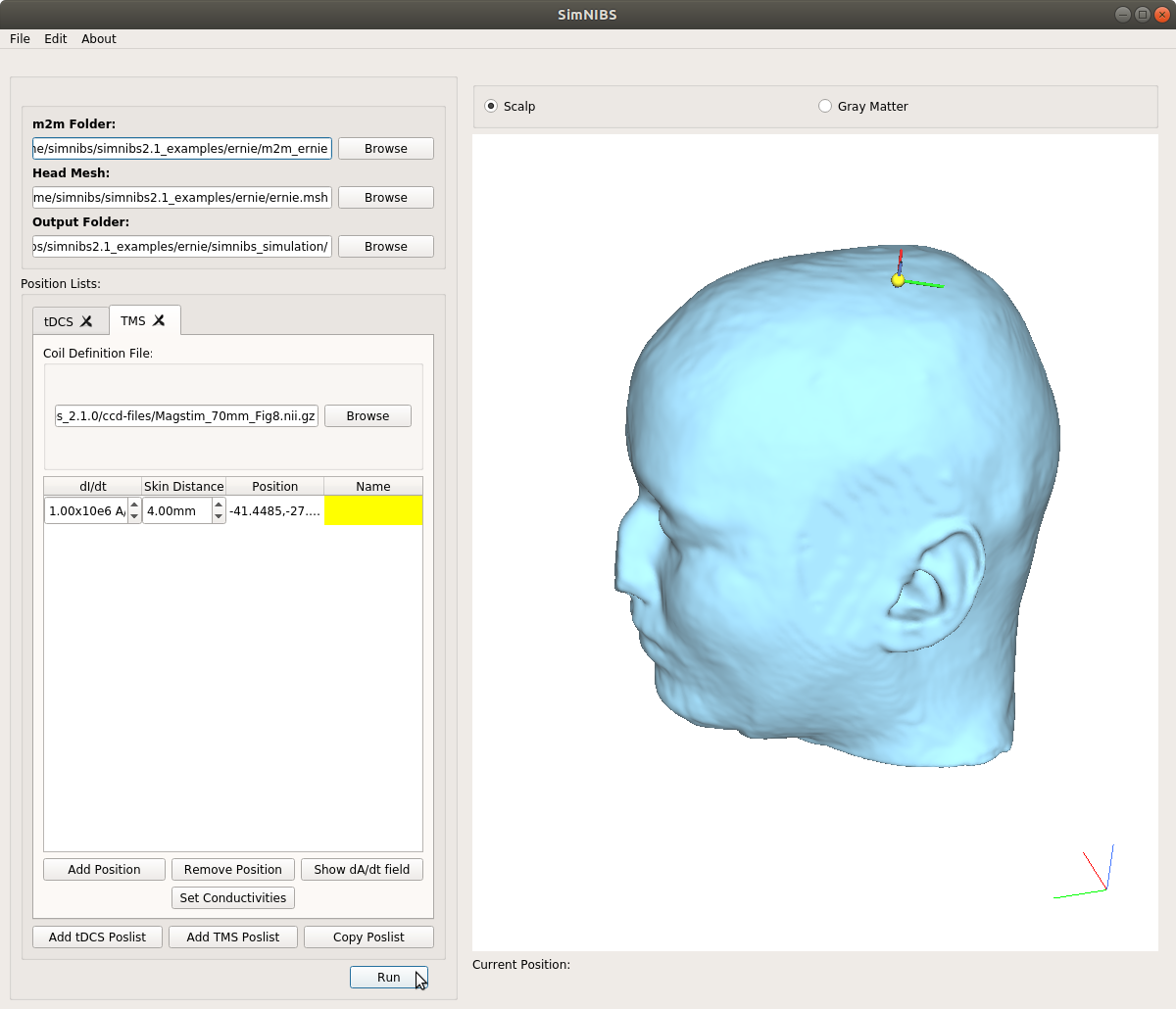
1. Launch the Graphical User Interface (GUI) from the Start Menu or by typing on a terminal window

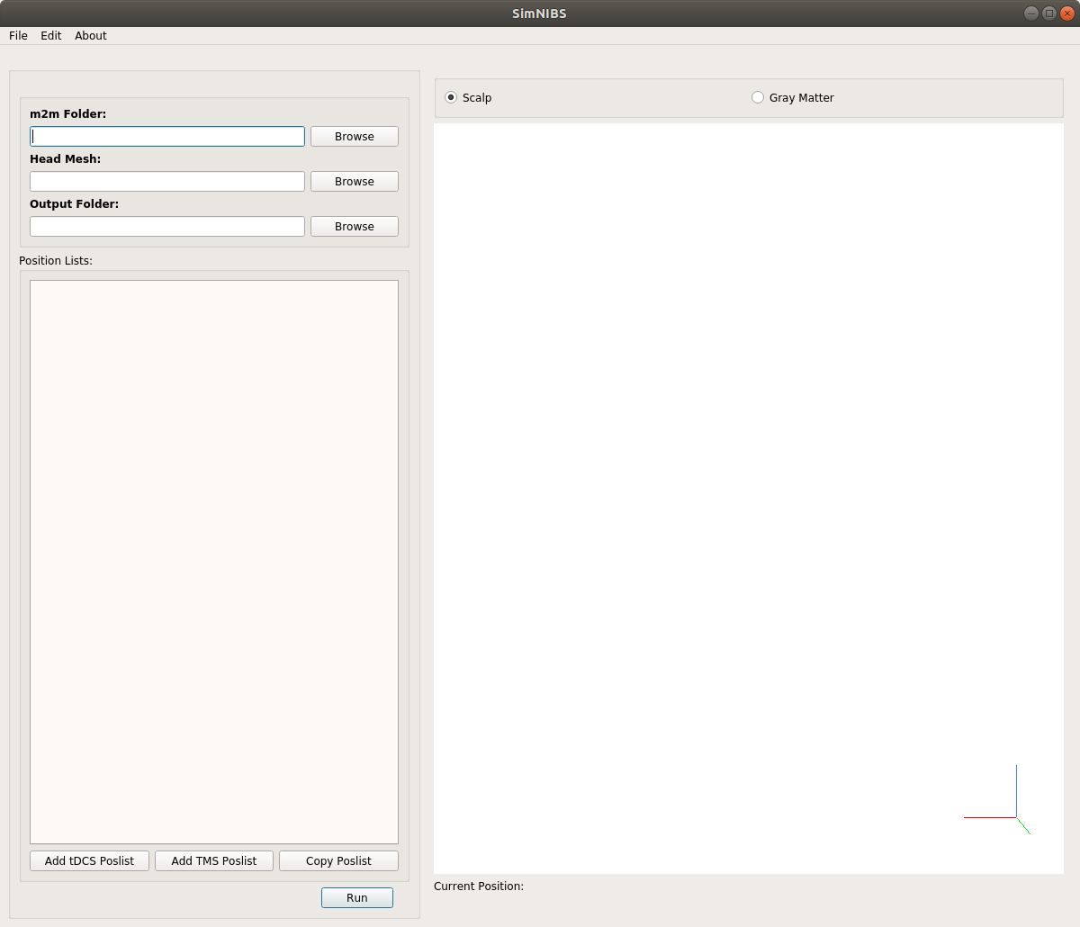
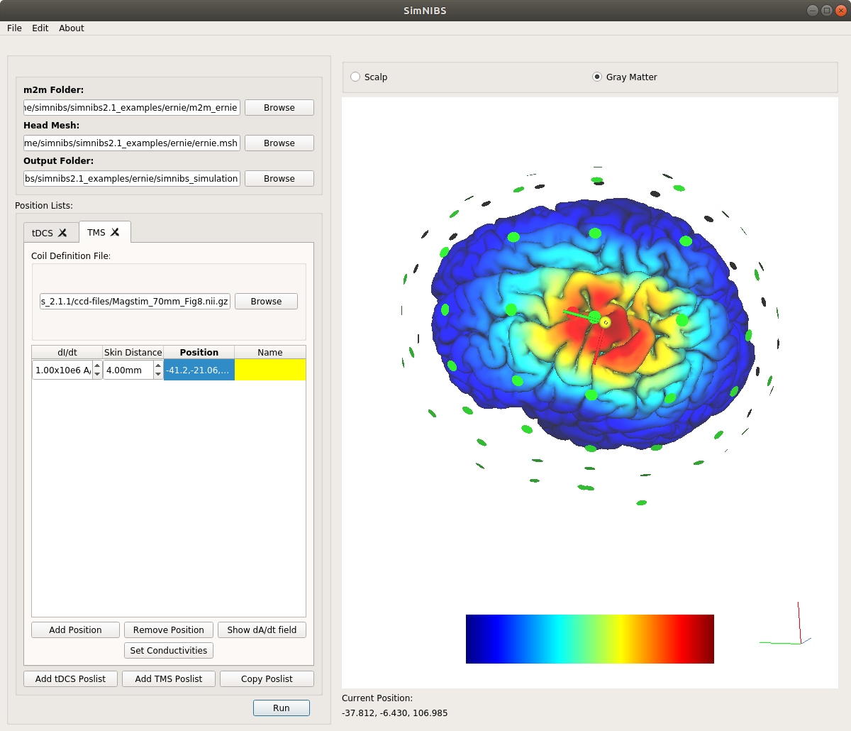
simnibs_gui

A window such as the following should appear:

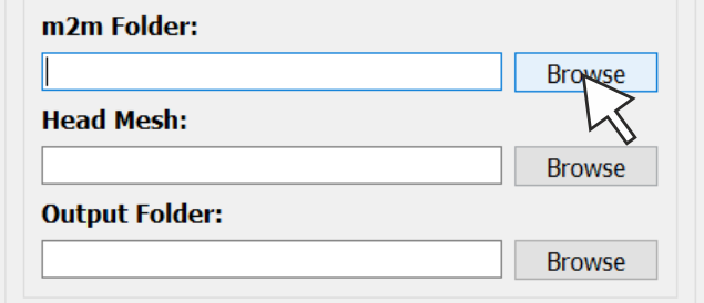
2. Click on the Browse button next to the m2m Folder box.

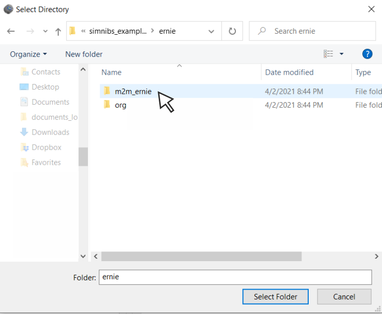
3. Navigate to the example dataset folder and select the m2m_ernie directory.

4. The head mesh will be loaded and the m2m Folder and Output Folder boxes filled.

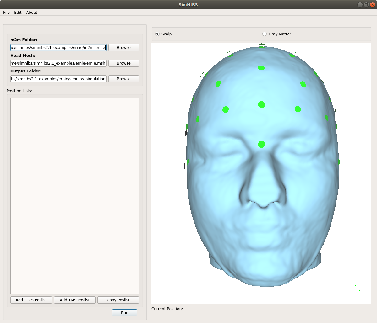
You can change the Output Folder by clicking on the Browse button close to it, and visualize the gray matter surface by clicking on the Gray Matter button above the head model.

Setting up a tDCS Simulation

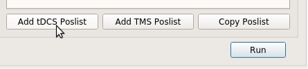
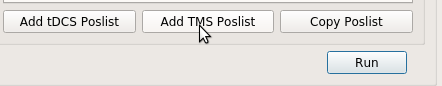
1. Click on Add tDCS Poslist at the bottom left of the window.

A new tab will show up.

2. Click on Add Electrode.

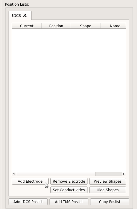
A new row will be shown in the table.

3. Click twice in the Shape cell.

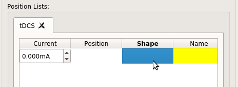
A new window will open where you can configure the electrode size and shape.

4. Let’s suppose we have a \(7.0 \times 5.5 \text{cm}^2\) electrode, composed of a single gel layer of 5 mm thickness.

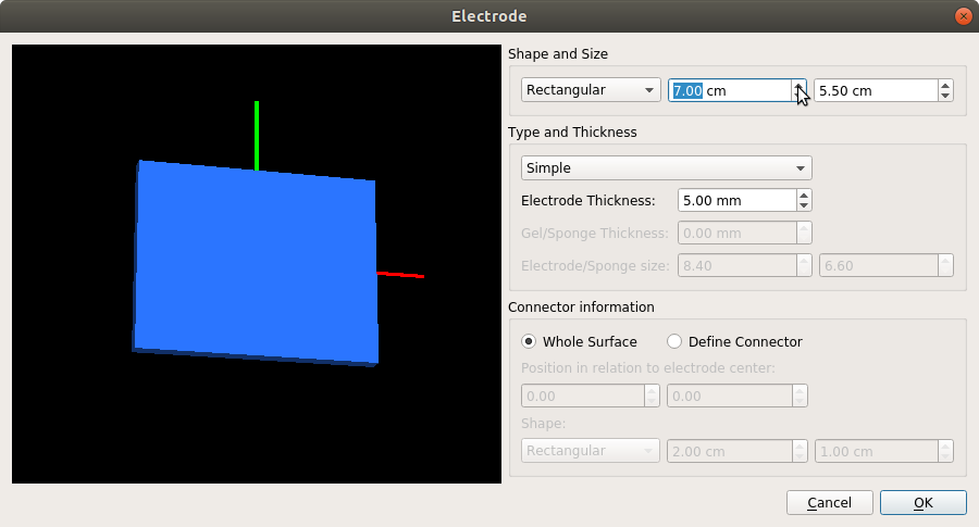
Please refer to the GUI documentation for a more detailed explanation of this window. You can also copy/paste electrode definitions by right-clicking in the shape cell.

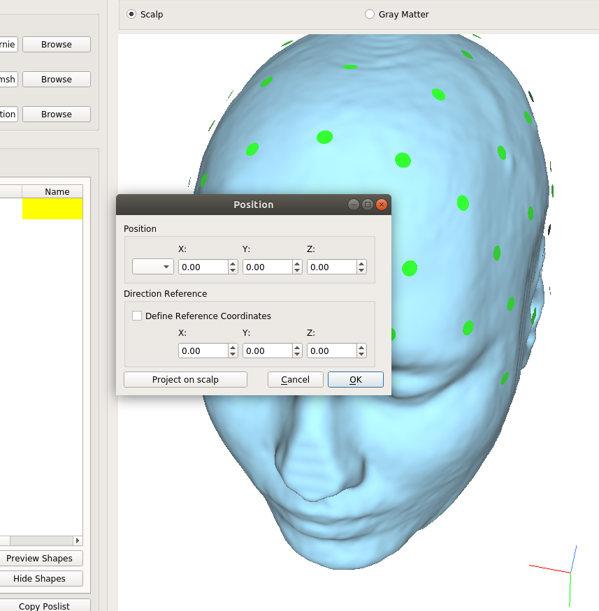
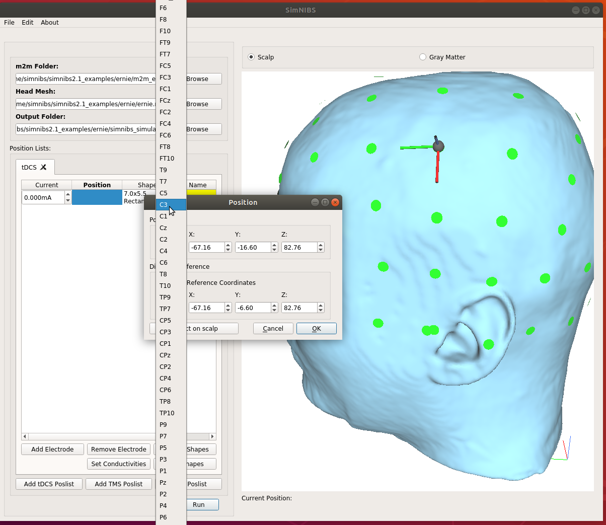
5. Now double-click in the Position cell. A new window will appear. You can either select an EEG position from the drop-down menu in the left or click twice in the model to get a position.

6. Choose the C3 electrode from the drop-down menu. A black sphere appears in the electrode position, with a green axis indicating the electrode’s “y” axis.

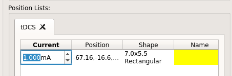
7. Select the electrode current in the first column of the electrode tables. Positive values designate anodes, and negative values cathodes. The sum of all current values has to be zero.

8. Now add a second electrode, place it at AF4 and double-click on a nearby position to rotate it, aligning the green axis with the top/down direction.

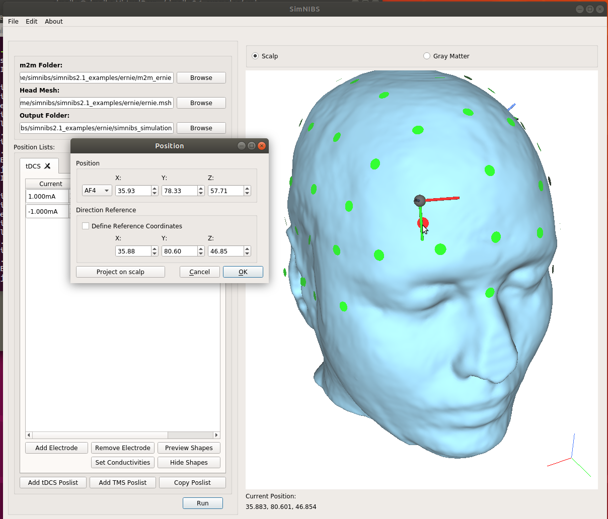
Select a shape and a current of \(-1.000 \text{mA}\) for this second electrode. You can see a simple preview of the electrode shapes by clicking on Preview Shapes at the bottom of the screen.

Setting up a TMS Simulation

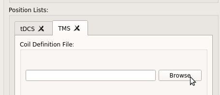
1. Click on Add TMS Poslist in the bottom of the window. A new TMS tab will be created.

2. Click on Browse and select the Magstim_70mm_Fig8.ccd coil file in the legacy_and_other subfolder

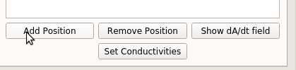
3. Click on Add Position.

4. Double-click in the Position cell.

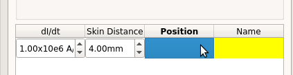
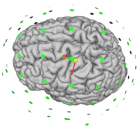
5. You can select the coil position the same way as an electrode position, or alternatively by double-clicking on the head model. In the TMS case, the y-axis (green) indicates the direction of the coil handle. Here, we will click on the Gray Matter button above the model window and place the coil above the motor cortex, with the green axis pointing anteriorly. This means that the coil handle points posteriorly. See here for more information on coil coordinates .

6. Additionally, you can also set the dI/dt (the current change ratio) and the coil-skin distance.

7. When using a .nii.gz coil file, click on Show dA/dt field to see the magnitude of the primary electric field.

Attention

This is NOT the electric field, but it can be interpreted as a very smooth approximation of it.

Note

Most coil files are supplied in .ccd-format, which needs less disk space compared to .nii.gz. However, the preview option Show dA/dt field in the GUI currently works only for .nii.gz coil file. If needed, you can use the command line tool ccd2nifti to convert coil files from .ccd to .nii.gz.

Setting Simulation Options

1. Go to Edit → Simulation Options.

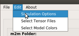
The following window will appear:

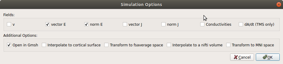
2. We can select the fields to be output from the simulation.

• v:

  Electrical Potential (Voltage). Units: Volts

• vector E:

  Electric field vector. Units: V/m

• magn E:

  Magnitude (or strength) of the electric field. Units: V/m

• vector J:

  Current density vector. Units: A/m²

• magn J:

  Magnitude of the current density. Units: A/m²

• Conductivities:

  Conductivity field. For isotropic conductivities, this is a scalar. For anisotropic conductivities, this is the largest eigenvector of the conductivity tensor. Units: S/m

• dA/dt:

  Primary field caused by the coil. TMS only. This is a vector field. Units: V/m

Select vector E and magn E.

3. We can also select Additional Options

• Open in Gmsh:

  Opens the simulation results in Gmsh

• Interpolate to cortical surface:

  Interpolates the fields along a surface at the center of the gray matter sheet. Not available for headreco models ran with --no-cat.

• Transform to fsaverage space:

  Interpolates to the middle of gray matter and transforms it to FsAverage space. Not available for headreco models ran with --no-cat.

• Interpolate to a nifiti volume:

  Interpolates the fields to a nifti volume.

• Transform to MNI space:

  Interpolates the fields to a nifti volume and applies a transformation to MNI space.

For the example run, we will select all of the above.

Running a Simulation

1. Click on Run at the bottom of the screen.

2. If there are no errors in the problem set-up, a new window will appear and show the simulation progress. The simulation takes a few minutes, and when finished a Gmsh window opens with the simulation results.

Now, please go on to our tutorial on Visualizing Results.

Output Files

After the simulation is finished, the simnibs_simulation directory will look like the following:

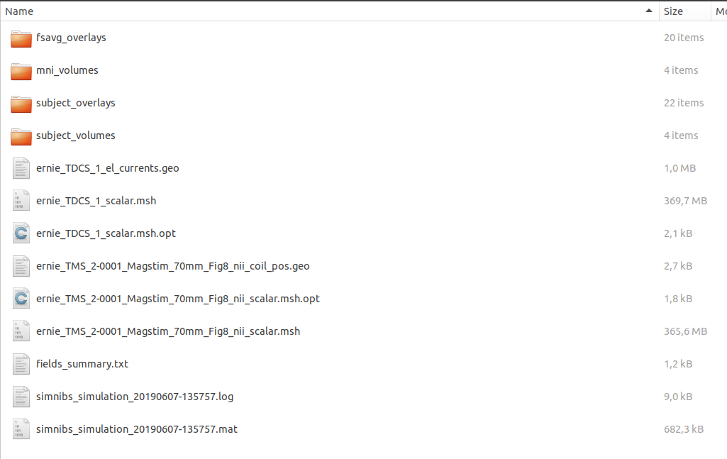
The main files here are the .msh files

• ernie_TDCS_1_scalar.msh

  With results of the tDCS simulation

• ernie_TMS_2-0001_Magstim_70mm_Fig8_nii_scalar.msh

  With results of the TMS simulation

The folders

• fsavg_overlays

• mni_volumes

• subject_overlays

• subject_volumes

are only present if the corresponding options are selected.

For a complete explanation of the output, please see Output Files .

Further Reading

For more information on the GUI, please see the SimNIBS 2.1 tutorial paper.