Leadfield-free TES Optimization
Note
When using this feature in a publication, please cite Weise K, Madsen KH, Worbs T, Knösche TR, Korshøj A, Thielscher A, A Leadfield-Free Optimization Framework for Transcranially Applied Electric Currents, bioRxiv 10.1101/2024.12.18.629095
Introduction
The leadfield-free TES optimization supports standard 2-channel TES, focal center-surround Nx1 TES, TI stimulation and Tumor Treating Fields (TTF). Several quantities of interest (QoI) are supported, including:
for TES: Electric field magnitude (“magn”) and its normal component relative to the cortex orientation (“normal”)
for TIS: maximal envelope of TI field magnitude (“max_TI”) and envelope of the normal component of the TI field (“dir_TI_normal”)
for TTF: Electric field magnitude (“magn”), whereby the field magnitudes of the two array pairs will be averaged
The following optimization goals are available:
Maximize the QoI in a region-of-interest
Optimize the intensity-focality tradeoff between the QoI in the region-of-interest and the QoI in an avoidance region (e.g. the rest of the brain)
Maximize the intensity of the QoI in the region-of-interest, while making the field as unfocal as possible. This can be relevant for TTF, where the aim is to focus the treatment on a tumor region, while maintaing high intensities throughout the brain (as the cancer cells might already have infiltrated further regions).
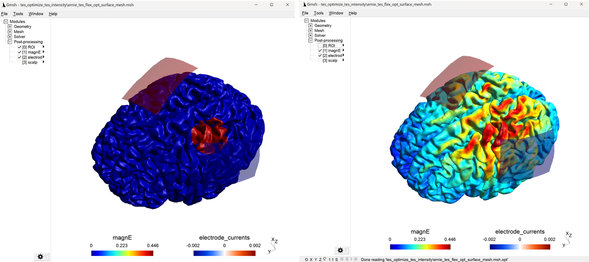
Example 1: Optimizing the electric field magnitude for 2-channel TES
This example maximizes the electric field strength in a ROI around the left hand knob.
Python
"""
Example to run TESoptimize with a standard TES montage to optimize the
field intensity in the ROI

Copyright (c) 2024 SimNIBS developers. Licensed under the GPL v3.
"""

from simnibs import opt_struct


""" Initialize structure """
opt = opt_struct.TesFlexOptimization()
opt.subpath = "m2m_ernie"  # path of m2m folder containing the headmodel
opt.output_folder = "tes_optimize_tes_intensity"

""" Set up goal function """
opt.goal = "mean"  # maximize the mean of field magnitude in the ROI
opt.e_postproc = "magn"  # postprocessing of e-fields ("magn": magnitude,
# "normal": normal component, "tangential": tangential component)

""" Define electrodes and array layout """
electrode_layout = opt.add_electrode_layout(
    "ElectrodeArrayPair"
)  # Pair of TES electrode arrays (here: 1 electrode per array)s
electrode_layout.length_x = [70]  # x-dimension of electrodes
electrode_layout.length_y = [50]  # y-dimension of electrodes
electrode_layout.dirichlet_correction_detailed = False  # account for inhomogenous current distribution at electrode-skin interface (slow)
electrode_layout.current = [0.002, -0.002]  # electrode currents

""" Define ROI """
roi = opt.add_roi()
roi.method = "surface"
roi.surface_type = "central"  # define ROI on central GM surfaces
roi.roi_sphere_center_space = "subject"
roi.roi_sphere_center = [
    -41.0,
    -13.0,
    66.0,
]  # center of spherical ROI in subject space (in mm)
roi.roi_sphere_radius = 20  # radius of spherical ROI (in mm)
# uncomment for visual control of ROI:
# roi.subpath = opt.subpath
# roi.write_visualization('','roi.msh')

""" Run optimization """
opt.run()
MATLAB
%
% Example to run TESoptimize with a standard TES montage to optimize the
% field intensity in the ROI
%
% Copyright (c) 2024 SimNIBS developers. Licensed under the GPL v3.
%

% Initialize structure
opt = opt_struct('TesFlexOptimization');
opt.subpath = 'm2m_ernie';                                % path of m2m folder containing the headmodel
opt.output_folder = 'tes_optimize_tes_intensity';

% Set up goal function
opt.goal = 'mean';                                        % maximize the mean of field magnitude in the ROI
opt.e_postproc = 'magn';                                  % postprocessing of e-fields ('magn': magnitude,
                                                          % 'normal': normal component, 'tangential': tangential component)

% Define electrodes and array layout
electrode_layout = opt_struct('ElectrodeArrayPair');      % Pair of TES electrode arrays (here: 1 electrode per array)
electrode_layout.length_x = [70];                         % x-dimension of electrodes
electrode_layout.length_y = [50];                         % y-dimension of electrodes
electrode_layout.dirichlet_correction_detailed = false;   % account for inhomogenous current distribution at electrode-skin interface (slow)
electrode_layout.current = [0.002, -0.002];               % electrode currents
opt.electrode = electrode_layout;

% Define ROI
roi = opt_struct('RegionOfInterest');
roi.method = 'surface';
roi.surface_type = 'central';                             % define ROI on central GM surfaces
roi.roi_sphere_center_space = 'subject';
roi.roi_sphere_center = [-41.0, -13.0,  66.0];            % center of spherical ROI in subject space (in mm)
roi.roi_sphere_radius = 20;                               % radius of spherical ROI (in mm)
opt.roi{1} = roi;
% uncomment for visual control of ROI:
% roi.subpath = opt.subpath;
% roi.fname_visu = 'roi';
% run_simnibs(roi)

% Run optimization
run_simnibs(opt)
The optimization will create the Gmsh output file ernie_tes_flex_opt_surface_mesh.msh with the ROI, the optimized field and the electrode positions. The optimized electrode positions are listed in the summary.txt. In addition, the results folder contains visualizations (electrode_channel…png) for control of the electrode array layouts.
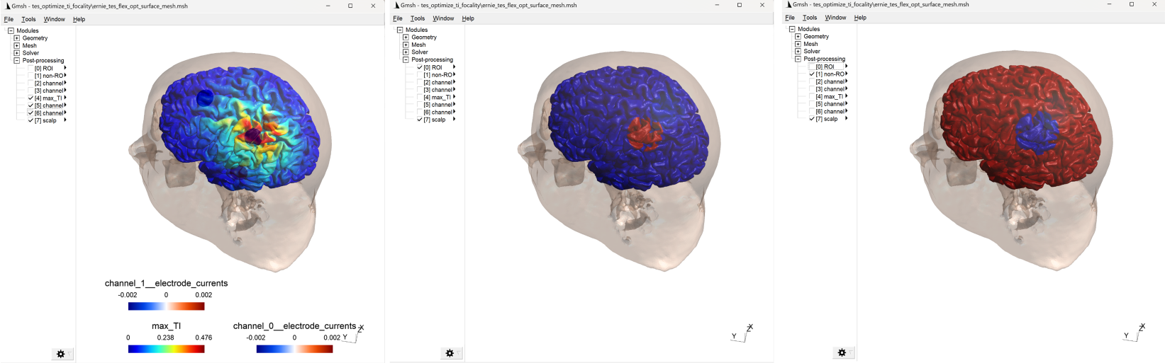
Example 2: Optimizing the focality of TI stimulation
This example optimizes the intensity - focality tradeoff of TIS, focused on the left hand knob. This requires the defintion of two regions: The first will be used as target ROI, the second will be the avoidance area (or “non-ROI). In addition, two thresholds are defined - the optimization goal is to ensure that the QoI (here: maxTI) is lower than the first threshold in the avoidance region, while it exceeds the second threshold in the ROI.
Python
"""
Example to run TESoptimize for Temporal Interference (TI) to optimize the
focality in the ROI vs non-ROI

Copyright (c) 2024 SimNIBS developers. Licensed under the GPL v3.
"""

from simnibs import opt_struct


""" Initialize structure """
opt = opt_struct.TesFlexOptimization()
opt.subpath = "m2m_ernie"  # path of m2m folder containing the headmodel
opt.output_folder = "tes_optimize_ti_focality"

""" Set up goal function """
opt.goal = "focality"  # optimize the focality of "max_TI" in the ROI ("max_TI" defined by e_postproc)
opt.threshold = [
    0.1,
    0.2,
]  # define threshold(s) of the electric field in V/m in the non-ROI and the ROI:
# if one threshold is defined, it is the goal that the e-field in the non-ROI is lower than this value and higher than this value in the ROI
# if two thresholds are defined, the first one is the threshold of the non-ROI and the second one is for the ROI
opt.e_postproc = "max_TI"  # postprocessing of e-fields
# "max_TI": maximal envelope of TI field magnitude
# "dir_TI_normal": envelope of normal component
# "dir_TI_tangential": envelope of tangential component
""" Define first electrode pair """
electrode_layout = opt.add_electrode_layout(
    "ElectrodeArrayPair"
)  # Pair of TES electrode arrays (here: 1 electrode per array)
electrode_layout.radius = [10]  # radii of electrodes
electrode_layout.current = [0.002, -0.002]  # electrode currents

""" Define second electrode pair """
electrode_layout = opt.add_electrode_layout("ElectrodeArrayPair")
electrode_layout.radius = [10]
electrode_layout.current = [0.002, -0.002]

""" Define ROI """
roi = opt.add_roi()
roi.method = "surface"
roi.surface_type = "central"  # define ROI on central GM surfaces
roi.roi_sphere_center_space = "subject"
roi.roi_sphere_center = [
    -41.0,
    -13.0,
    66.0,
]  # center of spherical ROI in subject space (in mm)
roi.roi_sphere_radius = 20  # radius of spherical ROI (in mm)
# uncomment for visual control of ROI:
# roi.subpath = opt.subpath
# roi.write_visualization('','roi.msh')

""" Define non-ROI """
# all of GM surface except a spherical region with 25 mm around roi center
non_roi = opt.add_roi()
non_roi.method = "surface"
non_roi.surface_type = "central"
non_roi.roi_sphere_center_space = "subject"
non_roi.roi_sphere_center = [-41.0, -13.0, 66.0]
non_roi.roi_sphere_radius = 25
non_roi.roi_sphere_operator = [
    "difference"
]  # take difference between GM surface and the sphere region
# uncomment for visual control of non-ROI:
# non_roi.subpath = opt.subpath
# non_roi.write_visualization('','non-roi.msh')

""" Run optimization """
opt.run()
MATLAB
%
% Example to run TESoptimize for Temporal Interference (TI) to optimize the
% focality in the ROI vs non-ROI
%
% Copyright (c) 2024 SimNIBS developers. Licensed under the GPL v3.
%

% Initialize structure
opt = opt_struct('TesFlexOptimization');
opt.subpath = 'm2m_ernie';                              % path of m2m folder containing the headmodel
opt.output_folder = 'tes_optimize_ti_focality';

% Set up goal function
opt.goal = 'focality';                                  % optimize the focality of 'max_TI' in the ROI ('max_TI' defined by e_postproc)
opt.threshold = [0.1, 0.2];                             % define threshold(s) of the electric field in V/m in the non-ROI and the ROI:
                                                        % if one threshold is defined, it is the goal that the e-field in the non-ROI is lower than this value and higher than this value in the ROI
                                                        % if two thresholds are defined, the first one is the threshold of the non-ROI and the second one is for the ROI
opt.e_postproc = 'max_TI';                              % postprocessing of e-fields
                                                        % 'max_TI': maximal envelope of TI field magnitude
                                                        % 'dir_TI_normal': envelope of normal component
                                                        % 'dir_TI_tangential': envelope of tangential component
% Define first electrode pair
electrode_layout = opt_struct('ElectrodeArrayPair');    % Pair of TES electrode arrays (here: 1 electrode per array)
electrode_layout.radius = [10];                         % radii of electrodes
electrode_layout.current = [0.002, -0.002];             % electrode currents
opt.electrode{1} = electrode_layout;

% Define second electrode pair
electrode_layout = opt_struct('ElectrodeArrayPair');
electrode_layout.radius = [10];
electrode_layout.current = [0.002, -0.002];
opt.electrode{2} = electrode_layout;

% Define ROI
roi = opt_struct('RegionOfInterest');
roi.method = 'surface';
roi.surface_type = 'central';                           % define ROI on central GM surfaces
roi.roi_sphere_center_space = 'subject';
roi.roi_sphere_center = [-41.0, -13.0,  66.0];          % center of spherical ROI in subject space (in mm)
roi.roi_sphere_radius = 20;                             % radius of spherical ROI (in mm)
opt.roi{1} = roi;
% uncomment for visual control of ROI:
% roi.subpath = opt.subpath;
% roi.fname_visu = 'roi';
% run_simnibs(roi)

% Define non-ROI
% all of GM surface except a spherical region with 25 mm around roi center
non_roi = opt_struct('RegionOfInterest');
non_roi.method = 'surface';
non_roi.surface_type = 'central';
non_roi.roi_sphere_center_space = 'subject';
non_roi.roi_sphere_center = [-41.0, -13.0,  66.0];
non_roi.roi_sphere_radius = 25;
non_roi.roi_sphere_operator = ['difference'];           % take difference between GM surface and the sphere region
opt.roi{2} = non_roi;
% uncomment for visual control of the ROI before running the optimization:
% non_roi.subpath = opt.subpath;
% non_roi.fname_visu = 'non-roi';
% run_simnibs(non_roi)

% Run optimization
run_simnibs(opt)
The optimization will create the Gmsh output file ernie_tes_flex_opt_surface_mesh.msh with the optimized field, electrode positions, ROI, and avoidance region. The optimized electrode positions are listed in the summary.txt. In addition, the results folder contains visualizations (electrode_channel…png) for control of the electrode array layouts.
Notes
The optimization uses the MKL Pardiso direct solver for accelerating the simulations. The SimNIBS standard FEM solver can be chosen optionally to reduce memory consumption, but will also substantially slow down the optimization.
32GB main memory are recommended, even thougth some optimizations will run with 16GB main memory.
Optimization is performed using the differential evolution algorithm, which is stochastic in nature. As such, solutions will differ between repeated optimization runs, even though the achieved final cost will be very close to each other.
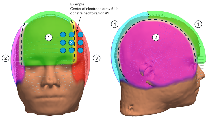
For TTF, we recommend setting constrain_electrode_locations to True, which will restrict the locations for each of the four electrode arrays to frontal, left and right parietal, and occipital. This speeds up the search by reducing the likelihood for overlapping configurations. The restriction is applied to the centers of the arrays, so that half of an array can still move into the neighboring skin areas, keeping sufficient flexibility for the optimization.
Please see TesFlexOptimization for a description of the option settings, RegionOfInterest for a description of the region-of-interest parameters, and Electrode and array layouts for TesFlexOptimization for a description of the electrode array layout parameters.