Group Analysis

SimNIBS supports group analysis of electric fields in both FsAverage and MNI spaces.

In this example, we will simulate the average electric field for a simple tDCS montage across five subjects using the FsAverage space.

Example Dataset

Click here to download the example dataset for group analysis.

This example dataset is composed of a subgroup of a cohort available at OpenfMRI. The data was processed in SimNIBS 4 using charm. For more information, please see the OSF repository and Saturnino et al., 2018.

In this example, we have five subjects, named sub01, sub09, sub10, sub12, and sub15. Their head models are stored in the corresponding m2m-folders m2m_sub01, m2m_sub09, etc.

Objective

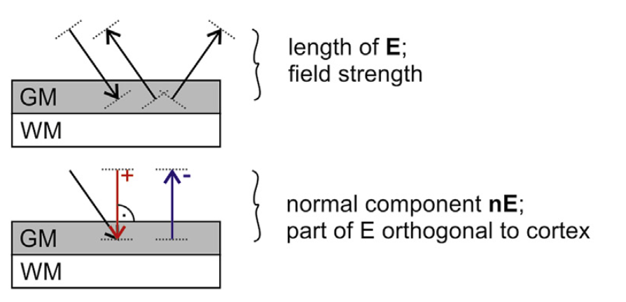
Suppose we apply tDCS on the five subjects using an anode over C3 and a cathode over AF4. We want to obtain the mean and standard deviation of the normal component of the electric field (that is, the incoming or outgoing electric field component) in the middle gray matter surface across all subjects.

Magnitude (aka Vector Norm) (top) and Normal (bottom) of the electric field, from Antonenko et al. 2019

Set up and Run Simulations

There are several ways to set-up and run Simulations in SimNIBS.

GUI

Set-up the simulation for each subject in the Graphical User Interface. In this case, remember to tick the Transform to FsAverage option in the Simulation Options Window. (under Edit -> Simulation Options)

Python

Write a Python script. In this case, remember to set map_to_fsavg to True in the SESSION structure. See Scripting Simulations for more information.

'''
    This example runs tDCS simulations with a bipolar montage for five subjects
    The dataset with the five head models is avaliable at https://osf.io/ah5eu/
    please look at the "group_average" for how to do a simple analysis of the group data
'''
import os
from simnibs import sim_struct, run_simnibs

# Set the subjects
subjects = ['sub01', 'sub09', 'sub10', 'sub12', 'sub15']

# Set a TDCSLIST structure with the simulation set-up
tdcslist = sim_struct.TDCSLIST()
tdcslist.currents = [0.001, -0.001]

anode = tdcslist.add_electrode()
anode.channelnr = 1
anode.centre = 'C3'
anode.pos_ydir = 'C1'
anode.shape = 'rect'
anode.dimensions = [50, 50]
anode.thickness = 4


cathode = tdcslist.add_electrode()
cathode.channelnr = 2
cathode.centre = 'AF4'
cathode.pos_ydir = 'F6'
cathode.shape = 'rect'
cathode.dimensions = [50, 70]
cathode.thickness = 4

# create main results folder
if not os.path.exists('bipolar'):
    os.mkdir('bipolar')

# Run the simulation in each subject
for sub in subjects:
    # ALWAYS create a new SESSION when changing subjects
    s = sim_struct.SESSION()
    s.map_to_fsavg = True
    s.map_to_MNI = True
    s.fields = 'eEjJ'
    s.subpath = 'm2m_' + sub
    s.pathfem = os.path.join('bipolar', sub)
    # Don't open in gmsh
    s.open_in_gmsh = False
    # Add the tdcslist we defined above
    s.add_poslist(tdcslist)
    # Run the sumulation
    run_simnibs(s)

MATLAB

Write a MATLAB script. In this case, remember to set map_to_fsavg to True in the SESSION structure. See Scripting Simulations for more information.

%  This example runs tDCS simulations with a bipolar montage for five subjects
%  The dataset with the five head models is avaliable at https://osf.io/ah5eu/
%  please look at the "group_average" for how to do a simple analysis of the group data

% Set the subjects
subjects = {'sub01', 'sub09', 'sub10', 'sub12', 'sub15'};

% Start a SESSION
S = sim_struct('SESSION');
S.map_to_fsavg = true;
S.map_to_MNI = true;
S.fields = 'eEjJ';

% Set a TDCSLIST with the simulation set-up
S.poslist{1} = sim_struct('TDCSLIST');
S.poslist{1}.currents = [0.001, -0.001];

S.poslist{1}.electrode(1).channelnr = 1;
S.poslist{1}.electrode(1).centre = 'C3';
S.poslist{1}.electrode(1).pos_ydir = 'C1';
S.poslist{1}.electrode(1).shape = 'rect';
S.poslist{1}.electrode(1).dimensions = [50, 50];
S.poslist{1}.electrode(1).thickness = 4;

S.poslist{1}.electrode(2).channelnr = 2;
S.poslist{1}.electrode(2).centre = 'AF4';
S.poslist{1}.electrode(2).pos_ydir = 'F6';
S.poslist{1}.electrode(2).shape = 'rect';
S.poslist{1}.electrode(2).dimensions = [50, 70];
S.poslist{1}.electrode(2).thickness = 4;

% create main results folder
if ~exist('bipolar','dir')
    mkdir('bipolar');
end

% Run the simulation in each subject
for i = 1:length(subjects)
     sub = subjects{i};
     S.subpath = fullfile(['m2m_' sub]);  % head mesh
     S.pathfem = fullfile('bipolar', sub); % Output directory
     run_simnibs(S);
end

Calculate Mean

When the simulations have finished, we need to collect their results to calculate an average. In SimNIBS, we can do it either in Python or MATLAB. Please notice: for setting up simulations, Python and MATLAB share a similar interface, but for post-processing, the interfaces can be very different.

Python

'''
    This example wil go throgh simulations and calculate
    the average and the standard deviation of the normal component
    of the electric field in FsAverage space

    It is a follow-up to the "run_simulations" example
'''
import os
import numpy as np
import simnibs

## Load simulation results
subjects = ['sub01', 'sub09', 'sub10', 'sub12', 'sub15']
results_folder = 'fsavg_overlays'
fsavg_msh_name = '_TDCS_1_scalar_fsavg.msh'
field_name = 'E_normal'

fields = []
for sub in subjects:
    # read mesh with results transformed to fsaverage space
    results_fsavg = simnibs.read_msh(
        os.path.join('bipolar', sub, results_folder, sub + fsavg_msh_name)
    )
    # save the field in each subject
    fields.append(results_fsavg.field[field_name].value)

## Calculate and plot averages
# Calculate
fields = np.vstack(fields)
avg_field = np.mean(fields, axis=0)
std_field = np.std(fields, axis=0)

# Plot
results_fsavg.nodedata = [] # cleanup fields
results_fsavg.add_node_field(avg_field, 'E_normal_avg') # add average field
results_fsavg.add_node_field(std_field, 'E_normal_std') # add std field

# show surface with the fields
results_fsavg.view(visible_fields='E_normal_avg').show()

## Calculate average in an ROI defined using an atlas
# load atlas and define a region
atlas = simnibs.get_atlas('HCP_MMP1')
region_name = 'lh.4'
roi = atlas[region_name]
# visualize region
results_fsavg.add_node_field(roi, region_name)
results_fsavg.view(visible_fields=region_name).show()

# calculate mean field using a weighted mean
node_areas = results_fsavg.nodes_areas()
avg_field_roi = np.average(avg_field[roi], weights=node_areas[roi])
print(f'Average {field_name} in {region_name}: ', avg_field_roi)
results_fsavg.add_node_field(roi, region_name)

MATLAB

% This example wil go throgh simulations and calculate
% the average and the standard deviation of the normal component
% of the electric field in FsAverage space
% 
% It is a follow-up to the "run_simulations" example

%% Load simulation results
subjects = {'sub01', 'sub09', 'sub10', 'sub12', 'sub15'};
results_folder = 'fsavg_overlays';
fsavg_msh_name = '_TDCS_1_scalar_fsavg.msh';
field_name = 'E_normal';

fields = {};
for i = 1:length(subjects)
    sub = subjects{i};
    % load mesh with results transformed to fsaverage space
    m = mesh_load_gmsh4(fullfile('bipolar', sub, results_folder, [sub fsavg_msh_name]));
    % Save the field of each subject
    fields{i} = m.node_data{get_field_idx(m, field_name, 'node')}.data;
end
%% Calculate and plot averages
% Calculate
fields = cell2mat(fields);
avg_field = mean(fields, 2);
std_field = std(fields, 0, 2);
% Plot
m.node_data = {}; %cleanup fields
m.node_data{1}.data = avg_field; % add average field
m.node_data{1}.name = [field_name '_avg'];
m.node_data{2}.data = std_field; % add std field
m.node_data{2}.name = [field_name '_std'];

% show surfaces with fields
mesh_show_surface(m, 'field_idx', [field_name '_avg'])
mesh_show_surface(m, 'field_idx', [field_name '_std'])

%% Calculate average in an ROI defined using an atlas
% load atlas and define a region
[m, snames]=mesh_load_fssurf('fsaverage','label','HCP_MMP1');
region_name = 'lh.4';
roi_idx=find(strcmpi(snames, region_name));
node_idx = m.node_data{end}.data==roi_idx;
% visualize region
m.node_data{end+1}.data = int8(node_idx);
m.node_data{end}.name = region_name;
mesh_show_surface(m, 'field_idx', region_name)

% calculate a weighted mean using the node areas
nodes_areas = mesh_get_node_areas(m);
avg_field_roi = sum(avg_field(node_idx).*nodes_areas(node_idx))/sum(nodes_areas(node_idx));
fprintf('Average %s in %s: %f\n', field_name, region_name, avg_field_roi)

Further Reading

For more information on group analysis, please see our SimNIBS 2.1 tutorial paper and Bungert et al. 2017.