Calculation of EEG Leadfields

Note

When using this feature in a publication, please cite Nielsen JD, Puonti O, Xue R, Thielscher A, Madsen KH (2023) Evaluating the influence of anatomical accuracy and electrode positions on EEG forward solutions. Neuroimage, 277:120259.

Currently, we support exporting leadfields for FieldTrip (MATLAB) and MNE-Python (python).

The general procedure for creating leadfields for electroencephalography (EEG) from a headmodel generated with SimNIBS includes the following steps

1. Run CHARM on the subject to create the anatomical model of the head. This creates the directory m2m_[subid]. Please see Creating Head Models for a more thorough description of this step.

2. Prepare EEG montage (electrode locations). In order to compute the leadfield, we need to place the EEG electrodes on our head model. This step transforms the electrode location information from FieldTrip or MNE-Python to SimNIBS and as such requires that you have electrode locations defined for your subject. This could be from digitizing the electrodes during an experiment or from warping a template to fit the subject. Therefore, we will use our software of choice (FieldTrip or MNE-Python) to compute a transformation that registers the EEG electrodes to subject MRI space and use prepare_eeg_montage to save these in a format that SimNIBS understands.

3. Prepare the TDCS leadfield. This step combines the data from step 1 and 2 to compute a TDCS leadfield. prepare_tdcs_leadfield is provided as a convenience function to run a TDCS leadfield simulation which forms the basis for the EEG forward solution computed by SimNIBS. This will compute the electric field and interpolate it to the central gray matter surface. By default, electrodes are modeled as points (projected onto the skin surface). Alternatively, electrodes can be modelled as circular with diameter of 10 mm and a thickness of 4 mm and meshed onto the head model. Default conductivities will be used. For more control, use the python function simnibs.eeg.forward.compute_tdcs_leadfield or define the simulation from scratch using simnibs.simulation.sim_struct.TDCSLEADFIELD.

4. Finally, we use prepare_eeg_forward to prepare the TDCS leadfield for EEG inverse calculations. This will also write the source space definition and (optionally) a “morpher” (i.e., a sparse matrix) mapping from subject space to fsaverage space.

FieldTrip

We will use the data from this FieldTrip tutorial. Download the mri data and the EEG data to the same directory. Extract the DICOM data. In MATLAB, we will assume that you are in this directory when executing the commands. Let us start by converting the MR image to NIfTI.

ft_defaults;

% convert dicom to nifti
mri = ft_read_mri(fullfile('dicom', '00000113.dcm'));
ft_write_mri('mri.nii.gz', mri.anatomy, 'transform', mri.transform , 'dataformat', 'nifti');

Then run CHARM to obtain the head model (mesh).

charm sub mri.nii.gz

This will create m2m_sub.

Attention

As you can see, mri.nii.gz is not ideal for making an accurate headmodel, however, it is OK for demonstration purposes.

Next, align electrodes with the MR image.

dataset = 'oddball1_mc_downsampled.fif';

elec = ft_read_sens(dataset, 'senstype', 'eeg');
elec = ft_convert_units(elec, 'mm');

% The dataset contains fiducials, however, I was not able to compute a
% good electrode-MRI registration using these

% shape   = ft_read_headshape(dataset, 'unit', 'cm');
% shape = ft_convert_units(shape, 'mm');

% Therefore, we will use the below transformation which I estimated
% interactively using `ft_electroderealign to align the electrodes
% and the MR image
head_to_mri_trans = [
    [1.0000    0         0         0];
    [0    1.0000         0   30.0000];
    [0         0    1.0000         0];
    [0         0         0    1.0000]
];

elec_mri = ft_transform_geometry(head_to_mri_trans, elec);

% Let us check the alignment

mesh = ft_read_headshape('m2m_sub/sub.msh');

figure;
hold on;
ft_plot_mesh(mesh, 'surfaceonly', 'yes', 'vertexcolor', 'none', ...
    'edgecolor', 'none', 'facecolor', 'skin', 'facealpha', 0.8);
camlight;
ft_plot_sens(elec, 'style', 'r');
ft_plot_sens(elec_mri, 'elecshape', 'sphere');
view([1 0 0]);

% Finally, save the transformed electrode positions
elec = elec_mri;
save('elec.mat', 'elec');

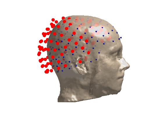
Coregistration result. Red is before transformation; blue is after.

Convert this to the format that SimNIBS uses for electrode positions

prepare_eeg_montage fieldtrip eeg_montage.csv elec.mat

This will create eeg_montage.csv which should contain the positions of the electrodes in subject MRI space. Now, compute the TDCS leadfield (subsample each hemisphere to 40,000 vertices).

prepare_tdcs_leadfield sub eeg_montage.csv -o fem_sub -s 40000

Finally, prepare it for EEG.

prepare_eeg_forward fieldtrip sub fem_sub/sub_leadfield_eeg_montage.hdf5 --fsaverage 40

We should now have the following files in the fem_sub directory

sub_leadfield_eeg_montage-40000-fwd.mat
sub_leadfield_eeg_montage-40000-morph.mat
sub_leadfield_eeg_montage-40000-src.mat

which can be used for source analysis with FieldTrip.

First, we process the EEG data as it is done here. (Note, that you need to download and put this file in your MATLAB path.) ft_rejectvisual will open a window where you can select bad trials based on variance.

% Read EEG data, segment, and preprocess
cfg = [];
cfg.dataset = dataset;
cfg.trialdef.prestim        = 0.2;
cfg.trialdef.poststim       = 0.4;
cfg.trialdef.rsp_triggers   = [256 4096];
cfg.trialdef.stim_triggers  = [1 2];
cfg.trialfun                = 'trialfun_oddball_stimlocked';

cfg = ft_definetrial(cfg);

cfg.continuous    = 'yes';
cfg.hpfilter      = 'no';
cfg.detrend       = 'no';
cfg.demean        = 'yes';
cfg.baselinewindow = [-inf 0];
cfg.dftfilter     = 'yes';
cfg.dftfreq       = [50 100];
cfg.lpfilter      = 'yes';
cfg.lpfreq        = 120;
cfg.channel       = 'EEG';
cfg.precision     = 'single';

data_eeg = ft_preprocessing(cfg);

% Remove bad trials

cfg = [];
cfg.method = 'summary';
cfg.keepchannel = 'no';
cfg.preproc.reref = 'yes';
cfg.preproc.refchannel = 'all';
data_eeg_clean = ft_rejectvisual(cfg, data_eeg);

% Apply an average reference

cfg = [];
cfg.reref = 'yes';
cfg.refchannel = 'all';
data_eeg_reref = ft_preprocessing(cfg, data_eeg_clean);

% Compute evoked response

% Evoked response incl. source covariance matrix
cfg = [];
cfg.covariance = 'yes';
cfg.covariancewindow = [0.08, 0.11];
timelock_eeg_all = ft_timelockanalysis(cfg, data_eeg_reref);

% cfg.trials = find(data_eeg_reref.trialinfo==1);
% timelock_eeg_std = ft_timelockanalysis(cfg, data_eeg_reref);
% cfg.trials = find(data_eeg_reref.trialinfo==2);
% timelock_eeg_dev = ft_timelockanalysis(cfg, data_eeg_reref);

% Compute noise covariance matrix
cfg = [];
cfg.covariance = 'yes';
cfg.covariancewindow = [-0.2, 0.0];
timelock_eeg_noise = ft_timelockanalysis(cfg, data_eeg_reref);

Contrary to the FieldTrip tutorial, we will not be fitting (two symmetric) dipoles as we cannot use the symmetry constraint with a leadfield from SimNIBS - and fitting a single dipole to this data probably does not make sense as the auditory stimulation is binaural. Instead, we will compute a minimum norm (distributed) source estimate.

Note

There are a few limitations on dipole estimates in FieldTrip when using a (precomputed) leadfield from SimNIBS. For example, the symmetry constraint and the nonlinear parameter search cannot be used as FieldTrip is not able to sample the leadfield at arbitrary locations (although, technically, this is possible, it is not currently supported).

load fem_sub/sub_leadfield_eeg_montage_subsampling-40000-fwd.mat
load fem_sub/sub_leadfield_eeg_montage_subsampling-40000-src.mat

fwd.tri = src.tri;

cfg               = [];
cfg.method        = 'mne';
cfg.sourcemodel   = fwd;
cfg.mne.prewhiten = 'yes';
cfg.mne.lambda    = 3;
cfg.mne.scalesourcecov = 'yes';
cfg.mne.noisecov = timelock_eeg_noise.cov;
source = ft_sourceanalysis(cfg, timelock_eeg_all);

Plot the estimated source power at 0.1 s after the presentation of the stimulus.

% the 76th time point correspondings to 0.1 s post simulus
m = source.avg.pow(:, 76);

figure;
ft_plot_mesh(source, 'vertexcolor', m);
view([0 90]);
h = light;
set(h, 'position', [0 1 0.2]);
lighting gouraud;
material dull;

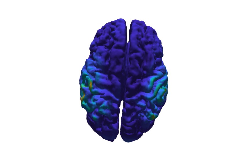
Minimum norm source estimate.

This is not perfect but it seems to align reasonably well with the symmetric dipole estimate from this section of the original FieldTrip tutorial.

MNE-Python

Attention

Currently, exporting forward solutions to MNE-Python is only compatible with MNE-Python <= 1.5.

First, make sure MNE-Python is installed in the same environment as SimNIBS. If you used the installer, you can call simnibs_python

simnibs_python -m pip install mne==1.5 h5io scikit-learn pyvistaqt

otherwise, ensure you are using the appropriate python interpreter and simply use python instead of simnibs_python (if you are using conda you can of course also install MNE-Python that way!). A miminal check that everything is working is simnibs_python -c "import mne, simnibs; print('OK')".

Next, download MNE-Python’s example data. We will use the data of the subject called sample. We start by converting the MRI T1.mgz to NIfTI (please set the correct path to the MNE example data).

from pathlib import Path

import nibabel as nib
import matplotlib.pyplot as plt
import numpy as np

import mne
from mne.coreg import Coregistration
from mne.io import read_info

mne_data_path = Path("/path/to/mne_data")

# this should download the data if not already present
data_path = mne.datasets.sample.data_path(mne_data_path)
subjects_dir = data_path / "subjects"
subject = "sample"

img = nib.load(subjects_dir / subject / "mri" / "T1.mgz")
nii = nib.Nifti1Image(img.get_fdata().astype(img.get_data_dtype()), img.affine)
# sets qform code to 2 which is fine
nii.set_qform(nii.affine)
nii.set_sform(nii.affine)
nii.to_filename("T1.nii.gz")

Then run CHARM. We use the --fs-dir option which grabs the cortical surfaces from a FreeSurfer run rather than estimate them as part of CHARM.

charm sample T1.nii.gz --forceqform --fs-dir /path/to/MNE-sample-data/subjects/sample

Perform coregistration using MNE-Python.

# This code is modified from the following MNE-Python tutorial on coregistration
# https://mne.tools/1.5/auto_tutorials/forward/25_automated_coreg.html

data_path = mne.datasets.sample.data_path(mne_data_path)
# data_path and all paths built from it are pathlib.Path objects
subjects_dir = data_path / "subjects"
subject = "sample"

fname_raw = data_path / "MEG" / subject / f"{subject}_audvis_raw.fif"
info = read_info(fname_raw)

eeg_indices = mne.pick_types(info, meg=False, eeg=True)
info = mne.pick_info(info, eeg_indices)

fiducials = "estimated"  # get fiducials from fsaverage
coreg = Coregistration(info, subject, subjects_dir, fiducials=fiducials)
coreg.fit_fiducials(verbose=True)
coreg.omit_head_shape_points(distance=5.0 / 1000)  # distance is in meters
coreg.fit_icp(n_iterations=20, nasion_weight=10.0, verbose=True)

dists = coreg.compute_dig_mri_distances() * 1e3  # in mm
print(
    f"Distance between HSP and MRI (mean/min/max):\n{np.mean(dists):.2f} mm "
    f"/ {np.min(dists):.2f} mm / {np.max(dists):.2f} mm"
)

# save the updated info object, i.e., containing only EEG electrodes
mne.io.write_info("info.fif", info)

_, _, mri_ras_t, _, _ = mne._freesurfer._read_mri_info(subjects_dir / subject / "mri" / "T1.mgz")
trans = mne.transforms.combine_transforms(coreg.trans, mri_ras_t, coreg.trans["from"], mri_ras_t["to"])

# The transformation is actually head <-> RAS but MNE-Python expects
# head <-> MRI (FreeSurfer surface RAS)
trans["to"] = coreg.trans["to"]

mne.write_trans('head_ras-trans.fif', trans)

Check the coregistration

plot_kwargs = dict(
    subject=subject,
    subjects_dir=subjects_dir,
    surfaces="head-dense",
    dig=True,
    eeg="original",
    meg=False,
    show_axes=True,
    coord_frame="head",
)
view_kwargs = dict(azimuth=45, elevation=90, distance=0.6, focalpoint=(0.0, 0.0, 0.0))

fig = mne.viz.plot_alignment(info, trans=coreg.trans, **plot_kwargs)
mne.viz.set_3d_view(fig, **view_kwargs)

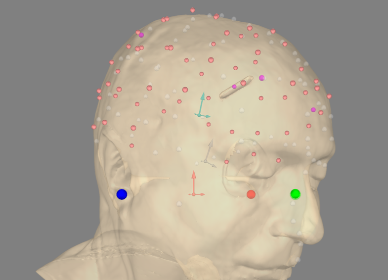
Coregistration result. Please note that what is visualized here is actually the electrodes transformed to FreeSurfer’s surface RAS space.

Convert the electrode location information to a format that SimNIBS understands (remember to insert correct paths).

prepare_eeg_montage mne eeg_montage.csv info.fif head_ras-trans.fif

This will create eeg_montage.csv which should contain the positions of the electrodes in subject MRI space.

Now, compute the TDCS leadfield.

prepare_tdcs_leadfield sample eeg_montage.csv -o fem_sample

Finally, prepare it for EEG.

prepare_eeg_forward mne sample fem_sample/sample_leadfield_eeg_montage.hdf5 info.fif head_ras-trans.fif --fsaverage 160

We should now have the following files in the fem_sample directory

MNE-Python

sample_leadfield_eeg_montage-fwd.fif
sample_leadfield_eeg_montage-morph.h5
sample_leadfield_eeg_montage-src.fif

for MNE-Python.

Source Analysis

Now, use the forward model that we just created to do source location with MNE-Python. The following is adapted from this tutorial to use EEG data and the forward model from SimNIBS.

fname_raw = data_path / "MEG" / "sample" / "sample_audvis_raw.fif"

raw = mne.io.read_raw_fif(fname_raw)
raw.pick_types(meg=False, eeg=True, stim=True, exclude=()).load_data()
raw.set_eeg_reference(projection=True)

events = mne.find_events(raw)
epochs = mne.Epochs(raw, events)
cov = mne.compute_covariance(epochs, tmax=0.0)
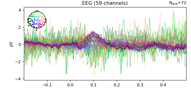
evoked = epochs["1"].average()  # trigger 1 in auditory/left
evoked.plot_joint()

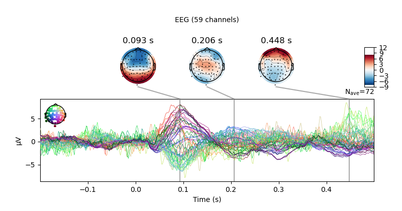
Evoked response with topo-plots.

Read forward solution, make inverse operator, and apply it.

# Read forward solution created with SimNIBS
fname_fwd = "fem_sample/sample_leadfield_eeg_montage-fwd.fif"
fwd = mne.read_forward_solution(fname_fwd)

method = "dSPM"

inv = mne.minimum_norm.make_inverse_operator(evoked.info, fwd, cov, verbose=True)
stc, residual = mne.minimum_norm.apply_inverse(evoked, inv, method=method, return_residual=True)

fig, ax = plt.subplots()
ax.plot(1e3 * stc.times, stc.data[::100, :].T)
ax.set(xlabel="time (ms)", ylabel="%s value" % method)
fig.show()

residual.plot()

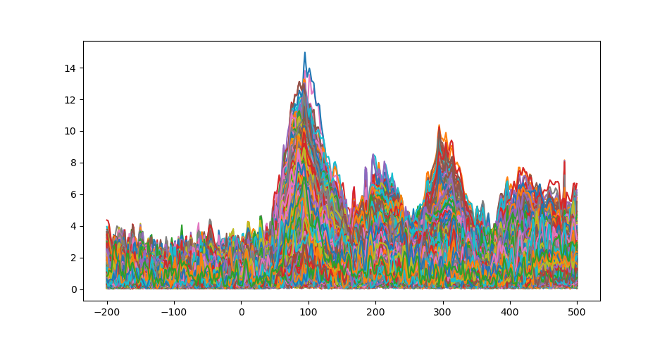
Time course of source estimates.

Residual of evoked response.

Plot the source time course and location. Note that this plot only works because we used --fs-dir with CHARM! Otherwise, the FreeSurfer and CHARM surfaces would differ and this function uses the FreeSurfer surfaces for plotting.

brain = stc.plot(subjects_dir=subjects_dir, initial_time=0.1)

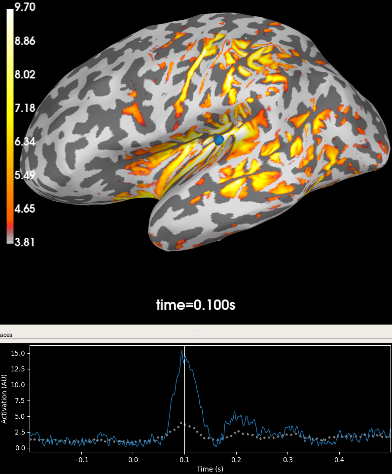
Source activation plottet on brain.

References

Nielsen JD, Puonti O, Xue R, Thielscher A, Madsen KH (2023) Evaluating the influence of anatomical accuracy and electrode positions on EEG forward solutions. Neuroimage, 277:120259.